Manish Shirke

By Manish Shirke
AI Systems Architect & DevOps Leader
Exploring the future of intelligent automation

Welcome. Today we will discuss about one of the most talked-about ideas in modern technology—neural networks—and break it down in plain developer language. If you’ve ever looked at research papers or AI blogs and felt buried in equations, don’t worry. By the end of this article, you’ll see that neural networks are built on concepts you already know: functions, loops, objects, and data transformations.

What Is a Neural Network?
Imagine you’re writing a function in Python. It takes an input, does some calculations, and gives an output. That’s all a neural network is—just a giant function. But here’s the twist: instead of you writing all the if-else statements or formulas, the network’s parameters—its weights and biases—are tuned using data until the function produces the right outputs.

Let’s compare:
• Traditional software: Rules + input → output.
• Neural networks: Data + output → rules.

For example, if you wanted to write a spam filter the old way, you’d write a set of rules:
• If the subject contains “free money,” mark as spam.
• If the sender is not in contacts, increase spam score.
• If there are ten exclamation marks, probably spam.

But the internet evolves faster than we can write rules. Neural networks solve this by automatically figuring out the “rules” from thousands of examples.
It’s like hiring a junior developer who reads all the code and figures out patterns—except this developer works with numbers, not words.

The Core Building Blocks
So what are these “neurons” people talk about? Forget biology for a second. A neuron in this context is just a small formula:

output = activation_function( weighted_sum_of_inputs )

Let’s unpack that:
• Inputs : These are the signals coming from the previous layer’s neurons or the initial data features.
• Weights: These are parameters or coefficients that the network learns during training. They determine the strength or importance of each input.
• Weighted Sum of Inputs : The core process starts with the weighted sum of inputs. If a neuron receives n inputs, x1​,x2​,…,xn​, each is multiplied by a corresponding weight, w1​,w2​,…,wn​, and then all are summed together.
• Bias: This is another learnable parameter which is a constant offset that adds flexibility and is typically added to this sum. It allows the neuron to shift the activation function (making it easier or harder to activate) regardless of the input’s value. 
• Mathematically, this intermediate result (often called the net input, or z) is: 
weighted_sum_of_inputs=z=(i=1∑n​wi​xi​)+b
• Activation function : The result of the weighted sum (z) is then passed through an activation function (σ). The Activation function introduces non-linearity into the network. Without it, the network would only be able to learn linear relationships, no matter how many layers it had. Common examples include ReLU (Rectified Linear Unit), Sigmoid, and Tanh.
output = σ( z ) 
• Output: This is the final value produced by the neuron, which then serves as an input to the neurons in the next layer, or as the final prediction.

In essence, the neuron first calculates a linear combination of its inputs (the weighted sum) and then applies a non-linear transformation (the activation function) to generate its final output.

If you’re a developer, this looks a lot like:
def neuron(inputs, weights, bias):
return activation(dot(inputs, weights) + bias)

That’s all! A neuron is just a little calculator that takes numbers in, multiplies, adds, and applies a function.

Now put a bunch of these neurons side by side—you get a layer.
Stack several layers—you get a network.
And when you stack many layers deep—that’s deep learning.

Networks as Composable Functions
Think of a neural network as nested function calls:
def network(x):
x = layer1(x)
x = layer2(x)
x = layer3(x)
return x

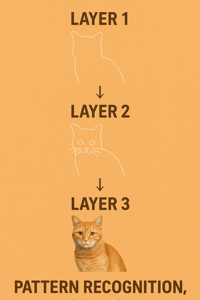
Each layer transforms the data a little bit. The first might extract rough patterns, like edges in an image. The middle layers refine them into shapes. The final layer says, “Aha, that’s a cat.”

If you’ve ever piped Unix commands together—cat file | grep error | sort—that’s basically how layers in a neural network work. Each one does a tiny transformation, and the magic comes from composition.

Training – The Learning Process
This is where things get interesting. How does a network actually learn?
1. Forward pass: Data flows in, output comes out.
2. Loss function: Compare output to the correct answer. Calculate error.
3. Backward pass (backpropagation): Work backwards to figure out which weights contributed to the error.
4. Weight update: Adjust weights slightly using an optimizer such as stochastic gradient descent (SGD) or Adam.

Now, what does that mean?
SGD: Think of it like climbing down a mountain in the fog. You don’t see the whole slope, but you can feel the steepest direction right under your feet and take one small step at a time. That’s stochastic gradient descent — it updates weights step by step using small random batches of data.
Adam: This is a smarter hiker with memory. Adam not only looks at the current slope but also remembers which directions worked well before, adjusting its step size adaptively. This makes training faster and more stable for many problems.
Repeat this process over thousands—or millions—of examples. Eventually, the network gets really good at predicting outputs.
For developers: imagine writing a program that auto-refactors itself every time a test fails. That’s exactly what a neural network does—except instead of code, it’s tweaking weights.

A Developer-Friendly Analogy
Think of weights as configuration values in a giant .env file.
• At the start, they’re all random. Your app won’t run properly.
• During training, you run tests, log failures, and tweak the values.
• After enough iterations, the config is dialed in, and the app runs smoothly.
Training is just automated config tuning at massive scale.

Why Neural Networks Are Powerful. Why bother with all this complexity?Because neural networks can represent nonlinear functions.
A linear model can only draw straight lines. That’s fine if your data is simple. But real life is messy—faces, voices, languages, stock prices.
By stacking nonlinear layers, neural networks can approximate insanely complex functions. That’s why they’re used in:
• Image recognition
• Speech to text
• Self-driving cars
• Large language models like ChatGPT

Most operations boil down to matrix multiplications and nonlinear functions — with special structures like convolutions or attention mechanisms layered on top.

A Small Code Example
Here’s a tiny network in PyTorch:
import torch.nn as nn
class TinyNet(nn.Module):
def __init__(self):
super(TinyNet, self).__init__()
self.fc1 = nn.Linear(10, 20)
self.fc2 = nn.Linear(20, 1)

def forward(self, x):
x = torch.relu(self.fc1(x))
x = torch.sigmoid(self.fc2(x))
return x

Explanation in plain words of the above code :
import torch.nn as nn allows access PyTorch’s neural network building blocks libraries.
The class TinyNet(nn.Module) inherits from nn.Module, which provides all the necessary functionality for tracking parameters, movement between devices, and training/evaluation modes.
The __init__(self) function is the constructor for the neural network class. Its purpose is to define and initialize all the layers and associated learnable parameters (weights and biases) that form the network’s structure. It calls the parent class constructor super(TinyNet, self).__init__() which is mandatory for any PyTorch module, as it properly initializes the parent class (nn.Module), allowing PyTorch to correctly track the network’s parameters and state. 
Then it defines the First Linear Layer 
self.fc1 = nn.Linear(10, 20)
It specifies that this layer expects 10 input features and will output 20 features. PyTorch automatically generates and initializes the 10×20 weight matrix and a bias vector of size 20, which are the parameters that the network will learn.
Then it defines the Second (Output) Linear Layer
self.fc2 = nn.Linear(20, 1)
It specifies that this layer takes the 20 features from the first layer’s output as input and produces 1 final output feature. This sets up the 20×1 weight matrix and a bias vector of size 1.
In summary, the __init__ method establishes the complete architecture(10→20→1) and reserves the necessary memory for all the parameters that will be adjusted during the training phase.
The forward(self, x) function is the most crucial part of a PyTorch neural network module. It defines the computational path or the flow of datathrough the network—how an input x is transformed into an output prediction. It is automatically called when you pass data to an instance of the network, like model(data).

The function takes an input tensor, x, and processes it sequentially through the defined layers and activation functions:
First Layer Processing : x = torch.relu(self.fc1(x)) 
The input data x (which has 10 features) is passed through the first fully connected (linear) layer, self.fc1. This performs the weighted sum of inputs and adds the bias (i.e., W1​x+b1​). The output is a tensor with 20 features. The resulting 20-feature output is immediately passed through the ReLU (Rectified Linear Unit) activation function torch.relu(). This introduces the necessary non-linearity that allows the network to learn complex patterns.

Second Layer Processing: x = torch.sigmoid(self.fc2(x))
The output from the previous First layer Processing step (now 20 features) is passed through the second fully connected layer, self.fc2. This performs its own weighted sum and bias addition (i.e., W2​(ReLU(…))+b2​). The output is a single feature (1-dimensional).
The final single-feature result is passed through the Sigmoid activation function torch.sigmoid()​. This function squashes the output into a range between 0 and 1 .

Output: return x
The function returns the final, processed output tensor, which is the network’s prediction .The output (a single value between 0 and 1)

That’s a complete network in under 15 lines. Notice how it looks like normal class-based OOP code. So, as a developer, don’t think of neural networks as alien objects. Think of them as libraries giving you a convenient abstraction over math.

Common Misconceptions
Before we wrap up, let’s clear the air:
• Neural networks are not magic. They’re just math and data.
• More layers ≠ better results. Bigger models are harder to train.
• They don’t “understand” like humans do—they just learn statistical patterns.
• Sometimes, simpler models like decision trees or even regex are faster and good enough.
Knowing when not to use a neural network is just as important as knowing how they work.

How Developers Should Think
Here’s the mental model I recommend:
• A neural network is a function that writes itself.
• Training is like unit testing at scale—failures guide improvements.
• Weights are just mutable state tuned over time.
• Frameworks like TensorFlow, PyTorch, and Keras are your standard libraries—don’t reinvent the wheel.

Closing Thoughts
So that’s neural networks explained—not from the lens of math, but from the lens of a developer. They’re not mystical. They’re just functions and layers, trained on massive amounts of data.